Dynamic windows in calculation groups

It is a function that can create a moving “window” above the input table and apply it to the computing context. That “window” is defined quite similarly, as it was in the case of the INDEX function. Or that the numerical representation of the position (0)1…X or X…-1(0) is used. But there is one fundamental difference. INDEX requires only one such representative, but the WINDOW function requires two.

Overall, the syntax can be confusing at first glance, so I’d rather spend some time on it:

Official documentation for WINDOWS function

Fascinating are the parameters “FROM” and “TO” and the mentioned “from_type” and “to_type.” This may be completely obvious to someone, but I have already had the honor of encountering the question. “From To? How is that direction meant?”

It all depends on the mentioned “type” parameters. There are precisely two values ​​that these parameters take:

• ABS
• REL

When you use the REL value, “FROM” or “TO” moves along the time axis with a positive number to the right and a negative one to the left. It is always a movement from the currently evaluated row of the input table. At the same time, the value 0 can be used for “FROM” or “TO” so that the just mentioned line is used as a “start” or “end” within the Window.

The ABS value is reminiscent of the INDEX function since 1 means the beginning of the input table/partition, and -1 the last line. The difference with INDEX (to remind you) is that WINDOW returns a range of rows, not just one row.

Of course, these “type” parameters can be combined so that you can have “ABS” for “FROM” and “REL” for “TO.” This is great for calculations of the YTD (Year-To-Date) type.

Let’s try it

For the DEMO, I will use the model I already used in the previous article regarding the INDEX function.

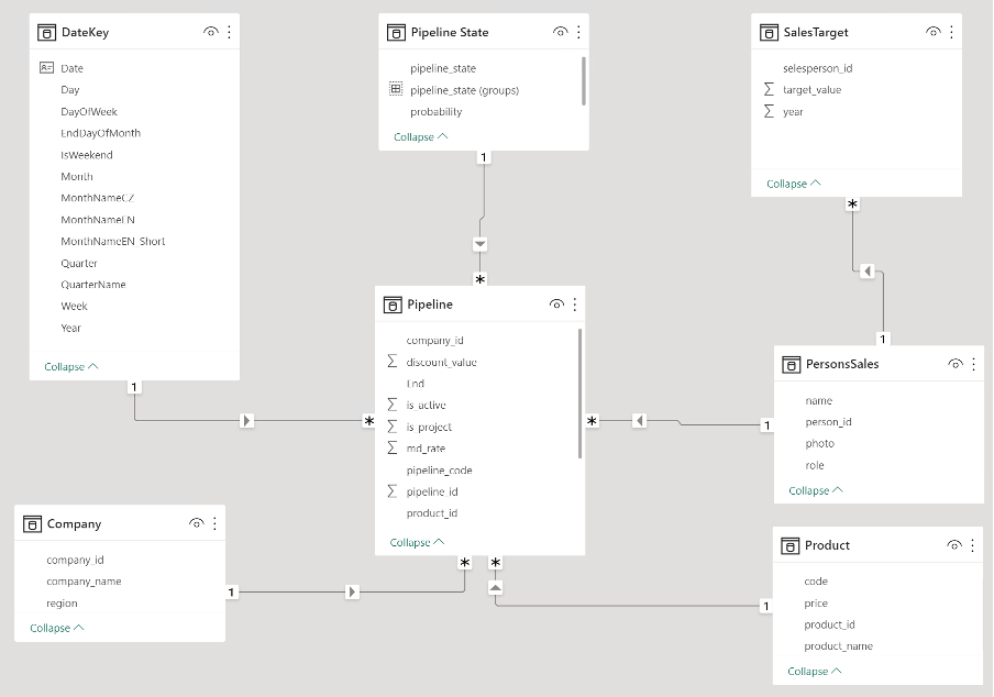Data model

And initial chart:

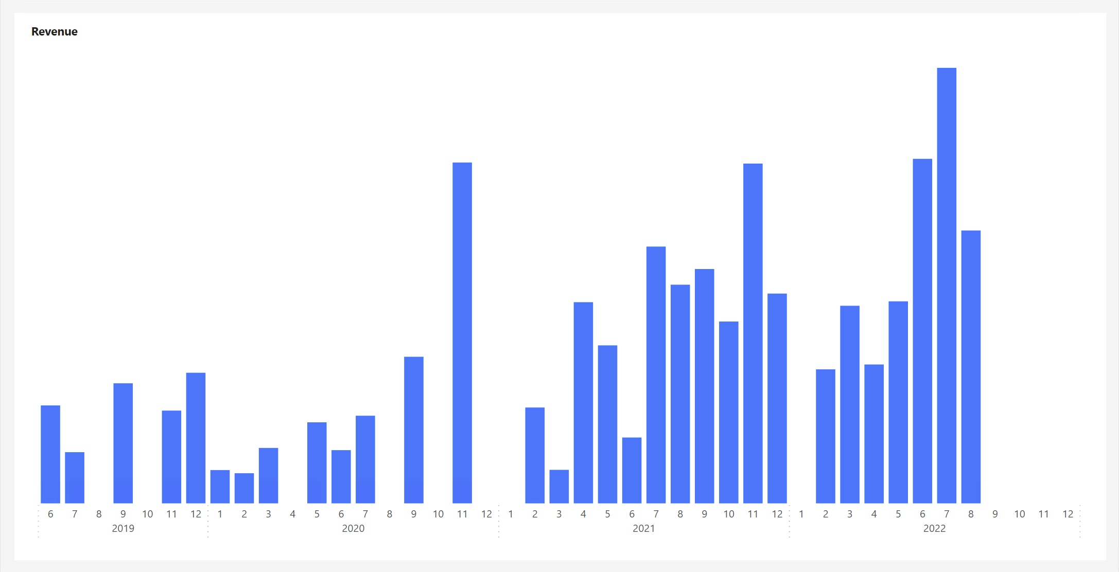Revenue

Here we have prepared a graph that contains the monthly results of Revenue. Of course, before the advent of the WINDOW function, we would do YTD equivalents using the TOTATYTD, DATESYTD, DATESBETWEEN, or FILTER functions, for example. But WINDOW should put these methods in its pocket.

Using WINDOW, it might look like this:

Within the function, I use the parameter FROM = 1 with TYPE = ABS, so I declare the Window from the beginning of the input table, and the parameter TO = 0 with TYPE = REL, so the Window ends with the current line. Without the PARTITIONBY function aimed at [Year], we would have a selected-period-to-date calculation. Because the PARTITIONBY function is present, it creates individual partitions in the specified table based on the specified input. In our case, based on individual years. So FROM = 1, TYPE = ABS will always be the first day of the currently executed Year. Not in the very first Year of the entire entry.

Which can be seen in the graph:

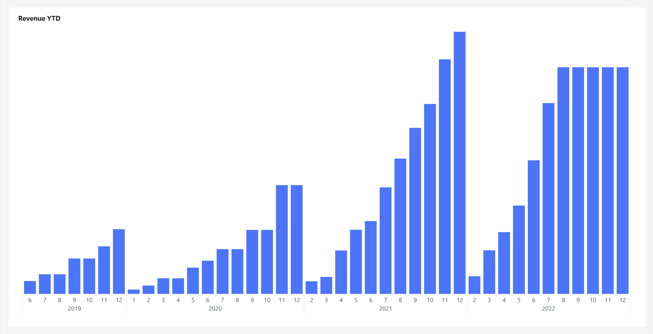Revenue YTD

At the same time, if we wanted to calculate the Year-End (YE) value in combination with PARTITIONBY, TYPE = ABS would help us in both cases. Both FROM = 1 and TO = -1. In short, it would set us back the whole Year.

We can also slightly modify the metric used, for example, to get a different but equally important calculation! Specifically, the Trailing Twelve-Month (T12M):

And the graph also beautifully reflected our change:

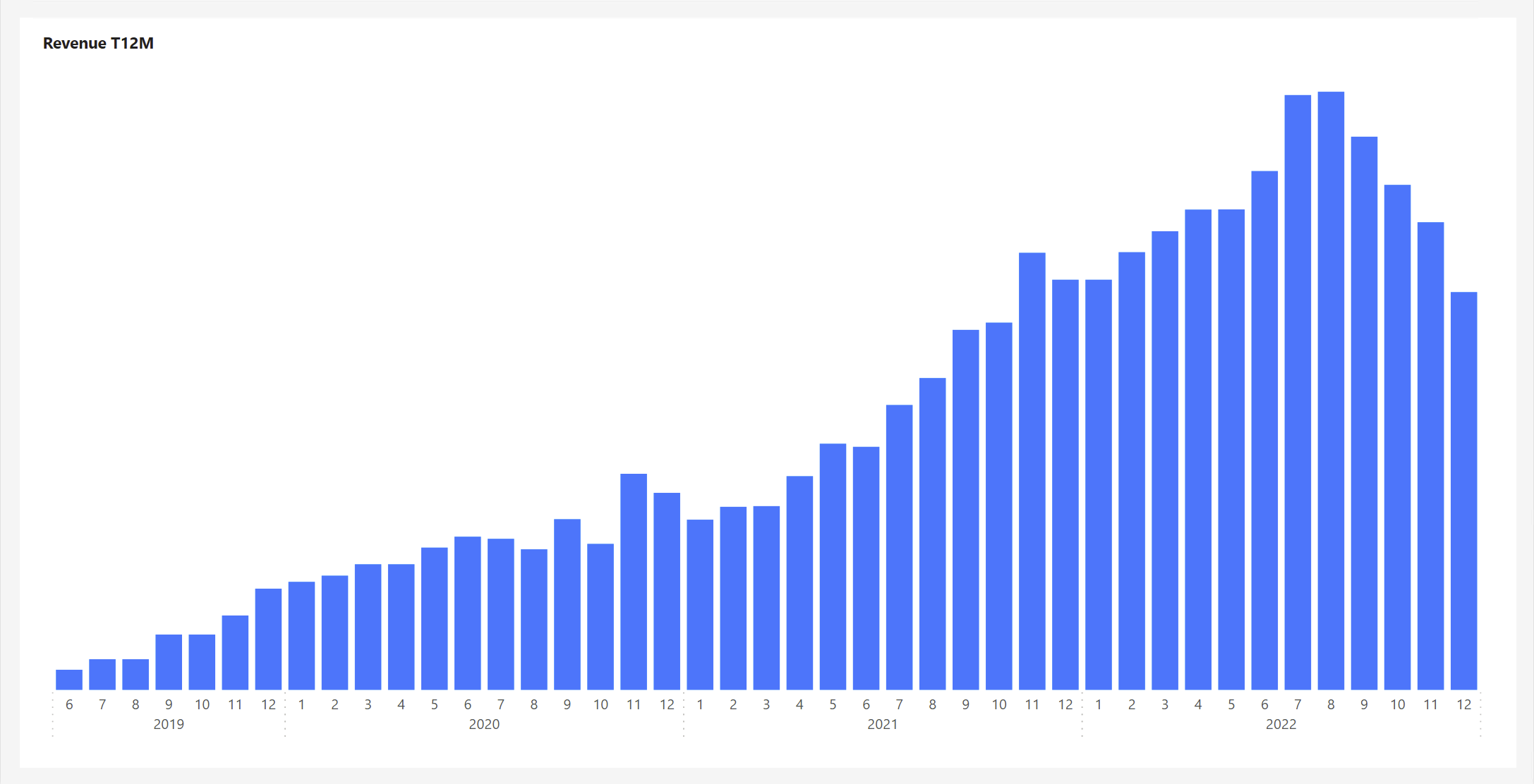Revenue T12M

Although it was only a tiny change in the metric, the result is entirely different and correct. In this, the WINDOW function is great, clear, and, above all, fast.

I often encounter the requirement that the user be able to switch between these types of calculations himself. As for switching to a single metric, we can solve it in different ways… quickly via a disconnected table. But what about dynamically? So that the user can, for example, select the metrics he wants to see via “Personalize your Visuals” or promote them inside the graph using Field of Measures. So we have to reach for Calculation Groups.

Cooperation with the Calculation Group

Let’s prepare three essential items on which we can test this behavior. We already have two in a way (they are mentioned above). First, we just replaced the measure with SELECTEDMEASURE().

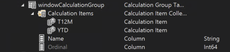Prepared Calculation Group

That last item will be selected-period-to-date (let’s give it an abbreviation like PTD):

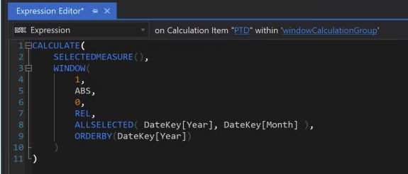Created PTD Calculation Item

Let’s load this calculation group of ours into the model and for now, let’s try to apply the last mentioned item using Slicer, for example, to check that everything works.

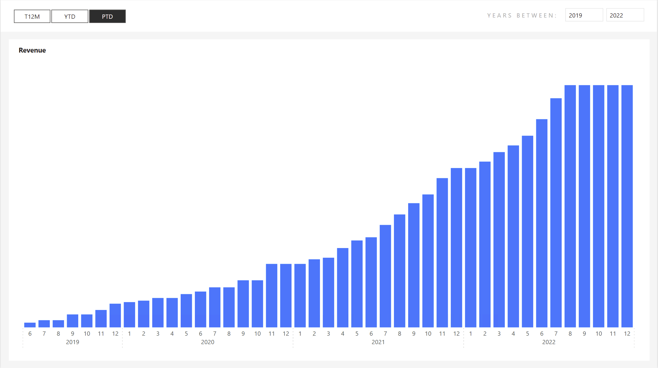PTD Item activated via Slicer

Everything works as expected, which is good news! I’m glad we didn’t run into any surprises. But let’s load it with Field of Measures.

I will create a fieldOfMeasures from three other measures, but they will have approximately similar Y-axis values. I really don’t want to mix apples and pears. So I selected Revenue, Pipeline Potential, and Costs:

Will the prepared expression in the calculation group be okay with it? To make the results more visible, I’ll switch from a bar chart to a line chart. After all, only three types of columns would probably not read very well with so many “categories” within the X-axis.

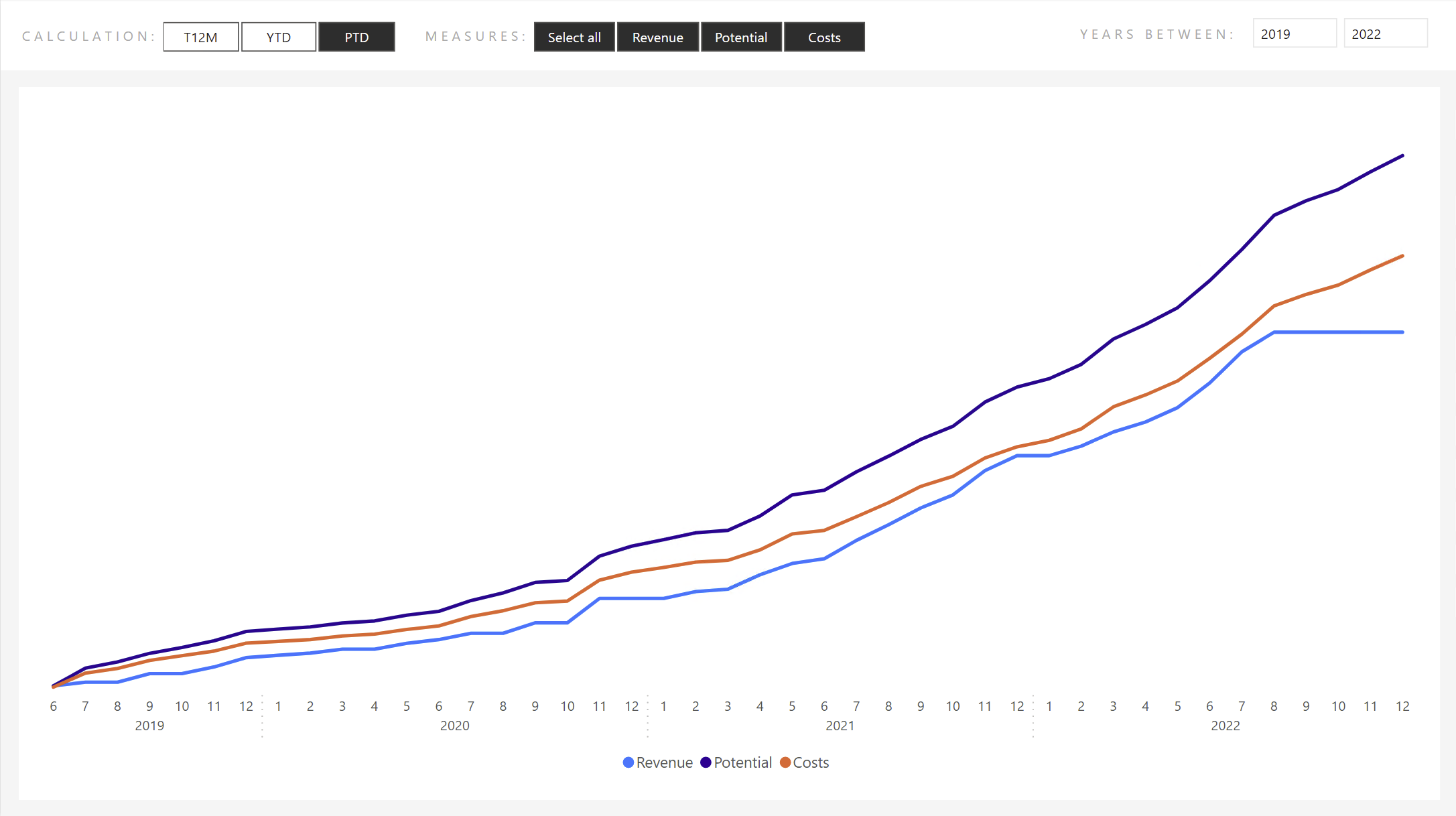Measures provided via Field Parameter modified by Calculation item with WINDOW function

No problem with that at all! I almost don’t want to believe it. I can also select only some parameters, and everything will recalculate correctly.

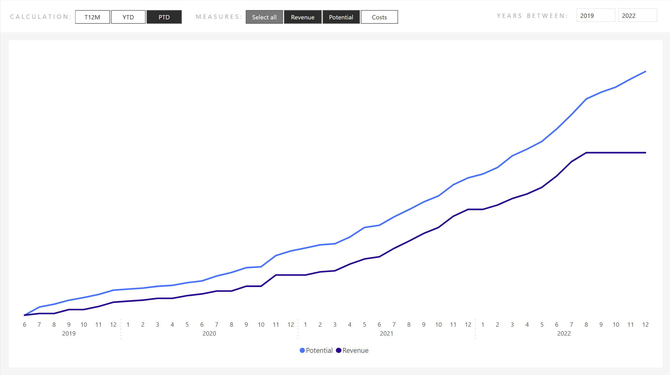Selected Revenue and Potential only

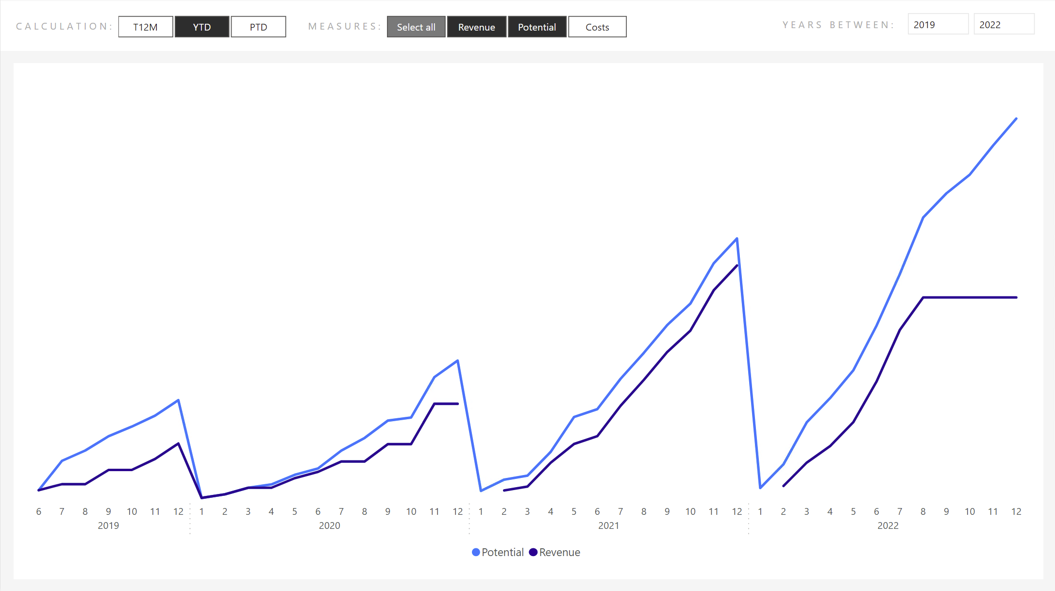YTD Calculation

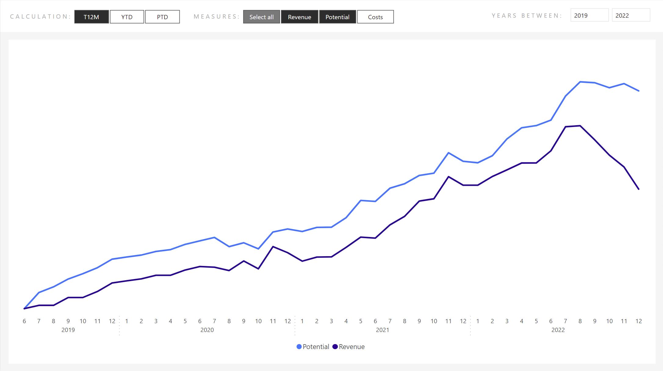T12M Calculation

Summary

During the tests, I did not encounter any major obstacle or specialty, such as the multiple movements of the OFFSET function. The WINDOW function is probably the most transparent and readable of all the newly added functions: (OFFSET, INDEX, WINDOW).

You will love the WINDOW function as much as I do, and it will become part of your regularly used functions.

If you are interested in any more information about WINDOW, I recommend the following links:

• Introducing DAX Window Functions (Part 1) – pbidax (wordpress.com)
• INTRODUCING DAX WINDOW FUNCTIONS (PART 2) – pbidax (wordpress.com)
• Unlock an ample new world by seeing through a window - Mincing Data - Gain Insight from Data (minceddata.info)
• Looking through the WINDOW - Calculating customer lifetime value with new DAX functions! - Data Mozart (data-mozart.com)